Learning ab initio phase-field models

Phase-field models derived from molecular dynamics, with the free-energy functional and mobility learned from ab initio data.

Mengyi Chen1 Peichen Zhong2,3 Zihan Zhang2 Qianxiao Li1,3,*

1Department of Mathematics, National University of Singapore

2Department of Materials Science and Engineering, National University of Singapore

3Institute for Functional Intelligent Materials, National University of Singapore

*Corresponding author

Key insights

Ab initio: grounded in microscopic theory

We derive the mesoscopic equation from a Mori–Zwanzig projection of molecular dynamics onto species-density fields under explicit assumptions, rather than postulating it.

Ab initio data, from MLIP-driven MD

We train on short molecular dynamics trajectories of a few thousand atoms, generated with machine-learning interatomic potentials of ab initio accuracy, without external potentials.

Learned from non-equilibrium dynamics

We learn from the dynamics of demixing and interface relaxation rather than from equilibrium sampling, which is data efficient and gives direct access to the spinodal region.

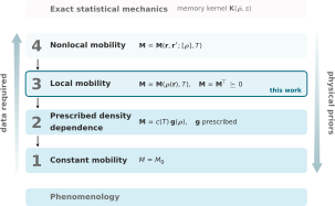
Free-energy functional and mobility, from systematic ladders

We select the free-energy functional and mobility from ladders of systematically improvable models, with their parameters learned jointly from the same dynamics.

Helium rain simulation

Ab initio in both derivation and learning

We develop ab initio phase-field (AIPF) models, grounded in microscopic theory and data. The term ab initio is used in the same spirit as in ab initio molecular dynamics (AIMD). In AIMD,

  1. the equations of nuclear motion follow from quantum mechanics under the Born–Oppenheimer approximation;
  2. the forces are computed using density functional theory, where the exchange–correlation functional is chosen from a ladder of systematically improvable approximations known as Jacob's ladder.

So what makes a phase-field model ab initio? Hover a column of the figure below.
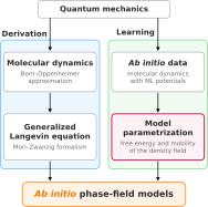
Panel a. Quantum mechanics at the top leads down two columns. Derivation: molecular dynamics under the Born–Oppenheimer approximation, then the generalized Langevin equation through the Mori–Zwanzig formalism. Learning: ab initio data from molecular dynamics with ML potentials, then model parametrization of the free energy and mobility of the density field. Both columns end in ab initio phase-field models.

Derivation and learning

Ab initio in both its derivation and its learning. Both start from quantum mechanics.

Hover a column.

Derivation

  1. Quantum mechanics to molecular dynamics under the Born–Oppenheimer approximation
  2. Molecular dynamics to a generalized Langevin equation through the Mori–Zwanzig formalism
  3. The generalized Langevin equation to the ab initio phase-field model under three assumptions
    • Markovian dynamics
    • Local mobility
    • Gaussian white noise

Learning

  1. MLIP-driven molecular dynamics of ab initio accuracy
  2. Free energy and mobility parametrized by neural networks, with their forms chosen from the ladders

The ladders

The excess free energy carries all interparticle correlations. From exact statistical mechanics down to phenomenology, each lower rung restricts its form further. Hover or tap a rung to see its functional form.
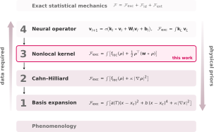
Panel b. A ladder of excess free-energy functionals between exact statistical mechanics at the top and phenomenology at the bottom. Rung 4, neural operator. Rung 3, nonlocal kernel, marked this work. Rung 2, Cahn–Hilliard. Rung 1, basis expansion. Data required grows towards the top and physical priors grow towards the bottom.
Each lower rung introduces additional restrictions, reducing flexibility and training-data requirements.

Exact statistical mechanics

F=Fexc+Fid+Fext\mathcal F=\mathcal F_{\mathrm{exc}}+\mathcal F_{\mathrm{id}}+\mathcal F_{\mathrm{ext}} Fid=kBT∑α∫ρα[ln⁡(ραΛα3)−1] dr,Fext=∫Vext⋅ρ dr\mathcal F_{\mathrm{id}}=k_{\mathrm B}T\sum_\alpha\int\rho_\alpha\big[\ln(\rho_\alpha\Lambda_\alpha^3)-1\big]\,\mathrm d\mathbf r,\qquad \mathcal F_{\mathrm{ext}}=\int\mathbf V_{\mathrm{ext}}\cdot\boldsymbol\rho\,\mathrm d\mathbf r

The ideal-gas part Fid\mathcal F_{\mathrm{id}} and the external-potential part Fext\mathcal F_{\mathrm{ext}} are known exactly, with Λα\Lambda_\alpha the thermal wavelength. The excess part Fexc\mathcal F_{\mathrm{exc}} accounts for interparticle interactions, and every rung below is an approximation of it.

Rung 4 · Neural operator

v0=ρ,vl+1=σ(kl∗vl+Wlvl+bl)\mathbf v_0=\boldsymbol\rho,\qquad \mathbf v_{l+1}=\sigma\big(\mathbf k_l\ast\mathbf v_l+\mathbf W_l\mathbf v_l+\mathbf b_l\big) Fexc=∫kL vL\mathcal F_{\mathrm{exc}}=\int\mathbf k_L\,\mathbf v_L

A neural operator, with layer fields vl\mathbf v_l, convolution kernels kl(r−r′,T)\mathbf k_l(\mathbf r-\mathbf r',T), channel-mixing weights Wl\mathbf W_l, biases bl(T)\mathbf b_l(T) and a pointwise nonlinearity.

Rung 3 · Nonlocal kernel this work

Fexc([ρ],T)=∫floc(ρ,T) dr+12∑αβ∬ρα(r) Wαβ(∣r−r′∣,T) ρβ(r′) dr dr′\begin{aligned}\mathcal F_{\mathrm{exc}}([\boldsymbol\rho],T)&=\int f_{\mathrm{loc}}(\boldsymbol\rho,T)\,\mathrm d\mathbf r\\&\quad+\frac12\sum_{\alpha\beta}\iint\rho_\alpha(\mathbf r)\,W_{\alpha\beta}(\lvert\mathbf r-\mathbf r'\rvert,T)\,\rho_\beta(\mathbf r')\,\mathrm d\mathbf r\,\mathrm d\mathbf r'\end{aligned}

Here flocf_{\mathrm{loc}} is a function of the local densities and WαβW_{\alpha\beta} the radial kernel between species α\alpha and β\beta. The kernel extends the square-gradient term of rung 2 to the full wavevector dependence of the pair correlations.

Rung 2 · Cahn–Hilliard

Fexc=∫[floc(ρ,T)+κ ∣∇ρ∣2] dr\mathcal F_{\mathrm{exc}}=\int\big[f_{\mathrm{loc}}(\boldsymbol\rho,T)+\kappa\,\lvert\nabla\boldsymbol\rho\rvert^2\big]\,\mathrm d\mathbf r

The Cahn–Hilliard square-gradient form with coefficient κ\kappa.

Rung 1 · Basis expansion

Fexc=∫[∑ncn(T) ϕn(x)+κ ∣∇x∣2] dr\mathcal F_{\mathrm{exc}}=\int\Big[\sum_n c_n(T)\,\phi_n(x)+\kappa\,\lvert\nabla x\rvert^2\Big]\,\mathrm d\mathbf r

A prescribed basis expansion in composition xx, with basis functions ϕn\phi_n such as Landau polynomials or Redlich–Kister terms and coefficients cn(T)c_n(T).

Two examples

Landau Fint=∫[a2(T−Tc)(xA−12)2+b (xA−12)4+κ2∣∇xA∣2] dr\mathcal F_{\mathrm{int}}=\int\Big[\tfrac a2(T-T_{\mathrm c})\big(x_A-\tfrac12\big)^2+b\,\big(x_A-\tfrac12\big)^4+\tfrac\kappa2\lvert\nabla x_A\rvert^2\Big]\,\mathrm d\mathbf r
Flory–Huggins Fexc=∫[w xA(1−xA)+κ2∣∇xA∣2] dr\mathcal F_{\mathrm{exc}}=\int\Big[w\,x_A(1-x_A)+\tfrac\kappa2\lvert\nabla x_A\rvert^2\Big]\,\mathrm d\mathbf r

Method

Three panels titled Simulation, Learning and Inference. Molecular dynamics with an ML potential produces configurations of species A and B. Their coarse-grained density fields feed a neural network that outputs a local mobility and a free-energy functional. The Inference panel shows thermodynamics, a free energy and phase diagram, and dynamics, a stochastic phase-field equation with snapshots of demixing over time.
  1. Data generation. Short molecular dynamics trajectories of small systems containing a few thousand atoms, driven by a machine-learning interatomic potential of ab initio accuracy, without external potentials. The trajectories start from unstable homogeneous mixtures or slabs and are coarse-grained into species-density fields.

  2. Training. The free energy and mobility, parametrized by neural networks, are learned jointly by matching the deterministic part of the mesoscopic equation to the measured evolution of the density fields,

    Ldyn=⟨∥∂tρ−∇⋅[Mθ∇μθ]∥H−12⟩.\mathcal L_{\mathrm{dyn}}=\Big\langle\Big\|\partial_t\boldsymbol\rho-\nabla\cdot\big[\mathbf M_\theta\nabla\boldsymbol\mu_\theta\big]\Big\|_{H^{-1}}^2\Big\rangle .

    Fluctuations in homogeneous equilibrium trajectories provide additional constraints on the mobility and the curvature of the free energy.

  3. Inference. The free energy alone gives the phase diagram. Together with the mobility, it gives fluctuating phase-field dynamics at length and time scales that molecular dynamics cannot reach without parallelization.

    Thermodynamics
    δFθδρ(r)=μ\frac{\delta\mathcal F_\theta}{\delta\boldsymbol\rho(\mathbf r)}=\boldsymbol\mu
    Dynamics
    ∂ρ∂t=∇⋅[Mθ∇δFθδρ]+∇⋅[2kBT Mθ  ξ]\frac{\partial\boldsymbol\rho}{\partial t}=\nabla\cdot\Big[\mathbf M_\theta\nabla\frac{\delta\mathcal F_\theta}{\delta\boldsymbol\rho}\Big]+\nabla\cdot\Big[\sqrt{2k_{\mathrm B}T\,\mathbf M_\theta}\;\boldsymbol\xi\Big]

Results

Binary Lennard-Jones mixture

A preliminary check of the framework on a symmetric binary Lennard-Jones mixture under overdamped Langevin dynamics. Below the critical temperature the mixture demixes spontaneously within the spinodal region. The AIPF model is compared with two rung 1 baselines, Landau and Flory–Huggins, trained on the same data with the same loss and mobility parametrization.

Three phase diagrams side by side: the AIPF model, the Landau baseline and the Flory–Huggins baseline, each with binodal, spinodal and critical temperature, against the MD binodal and critical temperature.
Thermodynamics (paper Fig. 3a, panels side by side). Binodal, spinodal and TcT_{\mathrm c} of the AIPF model and of the Landau and Flory–Huggins baselines against the MD binodal.

Dynamics

Domain size L(t) against time on a logarithmic axis from 0 to 10 000 tau for MD, AIPF, Landau and Flory–Huggins, three seeds each. MD and AIPF grow together to about 18 sigma, the two baselines stay well below.
Spinodal decomposition (paper Fig. 3b). Left, the composition field after a quench to T=1.20T=1.20, for molecular dynamics, the AIPF model and the two baselines, all from the same initial field. Each box is a single stochastic run. Right, the domain size L(t)L(t), three seeds each.

Iron–boron melt

FeB4 is predicted to be thermodynamically stable, but its synthesis has been reported only under high pressure. One route to solid-state synthesis proceeds through a transient melt at the interface between two solid precursors, which requires the melt at the target composition to be locally stable. A single AIPF model of the Fe–B melt is learned at 0, 5 and 10 GPa, and the curvature of its Gibbs free energy of mixing is quantified by the thermodynamic factor

Γ=xB(1−xB)kBT(∂2ΔGmix∂xB2)T,P,\Gamma=\frac{x_{\mathrm B}(1-x_{\mathrm B})}{k_{\mathrm B}T}\left(\frac{\partial^2\Delta G_{\mathrm{mix}}}{\partial x_{\mathrm B}^2}\right)_{T,P},

with Γ>0\Gamma>0 for a locally stable melt and Γ<0\Gamma<0 inside the spinodal region.

By learning from the dynamics, the AIPF model accesses the spinodal region directly, resolving the negative curvature inaccessible to equilibrium fluctuation measurements.

Four panels on the iron–boron melt: the thermodynamic factor over boron fraction and temperature at 0, 5 and 10 GPa with MD-classified states, the spinodal regions at the three pressures with FeB4 marked, the thermodynamic factor against boron fraction at three temperatures, and the model against MD for spinodal and unresolved states.
Paper Fig. 4.
  1. Γ(xB,T)\Gamma(x_{\mathrm B},T) at 0, 5 and 10 GPa, with the MD classification of the sampled states.
  2. The spinodal regions at the three pressures. The star marks FeB4 at 1500 K, inside the spinodal region at 0 and 5 GPa and outside it at 10 GPa.
  3. Γ(xB)\Gamma(x_{\mathrm B}) at three temperatures for each pressure. Dots mark the FeB4 composition.
  4. The model against MD for states that MD classifies as spinodal or unresolved. The model agrees with the spinodal classification and predicts the sign of Γ\Gamma for unresolved states.

Hydrogen–helium under planetary conditions

Hydrogen–helium mixtures make up most of the mass of gas giants such as Jupiter and Saturn. Inside them, helium is hypothesized to become immiscible in metallic hydrogen and settle as droplets toward the planetary center, a process known as helium rain. Whether and where it occurs depends on the immiscibility boundary, and its evolution on the kinetics of droplet nucleation, growth and transport. A single AIPF model spans 200 to 800 GPa and 2000 to 12 000 K.

Thermodynamics

The hydrogen–helium binodal surface in temperature, helium fraction and pressure, with its critical line, and two MD snapshots: a mixed state outside the two-phase region and a demixed slab inside it.
Binodal surface (paper Fig. 5a) with its critical line Tc(P)T_{\mathrm c}(P), and MD snapshots of a mixed state and a demixed slab.
Isobaric sections of the hydrogen–helium phase diagram at 200, 400, 600 and 800 GPa, binodal and spinodal with the critical temperature of each, and MD points at 800 GPa.
Isobaric sections (paper Fig. 5b). Binodal and spinodal at 200, 400, 600 and 800 GPa, with MD points at 800 GPa.

Helium rain in gas giants

Schematic wedge of a gas giant: molecular hydrogen, the helium-rain layer, metallic hydrogen and a dilute core.
Where it rains (paper Fig. 5c). The helium-rain layer in a gas giant.
The demixing temperature against pressure at a fixed helium fraction compared with published boundaries.
Against published boundaries (paper Fig. 5d). The learned binodal and spinodal along the pressure axis next to earlier predictions.
Binodal and spinodal against pressure with the interior temperature profiles of Jupiter and Saturn.
Jupiter and Saturn (paper Fig. 5e). The learned binodal and spinodal against the interior profiles of both planets.

The model captures droplet nucleation and growth in helium-rain simulations of a domain corresponding to 2.2 million atoms, far beyond the scale of atomistic modeling at comparable accuracy.

Dynamics simulation

Five snapshots of a helium-rain simulation from 20 to 1000 ps: droplets nucleate, grow, settle under gravity and form a helium layer at the bottom of the column, shown as droplet surfaces coloured by radius and as the helium fraction on the column faces.
Nucleation, growth and settling (paper Fig. 5f,g). Helium rain in a hydrogen–helium column at 400 GPa, 3700 to 3900 K along the planetary temperature gradient, corresponding to 2.2 million atoms. Snapshots at 20 to 1000 ps, with droplets coloured by radius and the helium fraction on the faces of the column. The full simulation plays beside the key insights above.

Citation

If you use this code, please cite the paper.

@article{chen2026aipf,
  title   = {Learning ab initio phase-field models},
  author  = {Chen, Mengyi and Zhong, Peichen and Zhang, Zihan and Li, Qianxiao},
  journal = {arXiv preprint arXiv:2610.01432},
  year    = {2026},
  doi     = {10.48550/arXiv.2610.01432},
  url     = {https://arxiv.org/abs/2610.01432}
}